Shear and Moment Diagrams

Introduction

Shear force and bending moment diagrams describe how internal forces and moments vary along a beam due to applied loads and reactions. These diagrams are essential for understanding how beams deform and where maximum internal stresses occur. Shear and moment relationships are found using equilibrium equations and section cuts.

General Procedure

1. Draw the free-body diagram.

2. Solve support reactions using $\Sigma F_{y} = 0$, $\Sigma F_{x} = 0$, and $\Sigma M = 0$.

3. Divide the beam into regions between loads.

4. Cut the beam within each region.

5. Apply equilibrium equations to solve for $V(x)$ and $M(x)$ in every region.

6. Plot values of shear and moment.

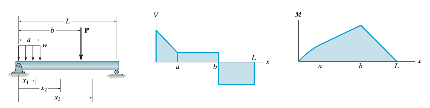
Key Relationships Between Load, Shear, and Moment

$w(x) = \frac{dV}{dx}$ or $V(x) = \int_{}^{}w(x)$

The slope of a shear diagram equals the negative of the distributed load.

(i.e. positive distributed load downward → shear decreases)

$V(x) = \frac{dM}{dx}$ or $M(x) = \int_{}^{}V(x)$

The slope of the moment diagram equals the shear.

(i.e. positive shear → moment increases)

Think of these as a chain: $w(x)$ → $V(x)\$→ $M(x)$

Shape Relationships

No load → constant shear → linear moment

Uniform load → linear shear → parabolic moment

Changing load → parabolic shear → cubic moment

Important Diagram Rules

Point Loads

• Cause a sudden jump in shear

• Do not cause a jump in moment

Applied Moments

• Cause a sudden jump in moment

• Do not change shear

Maximum Moment

• Occurs where $V(x) = 0$

Example 1:

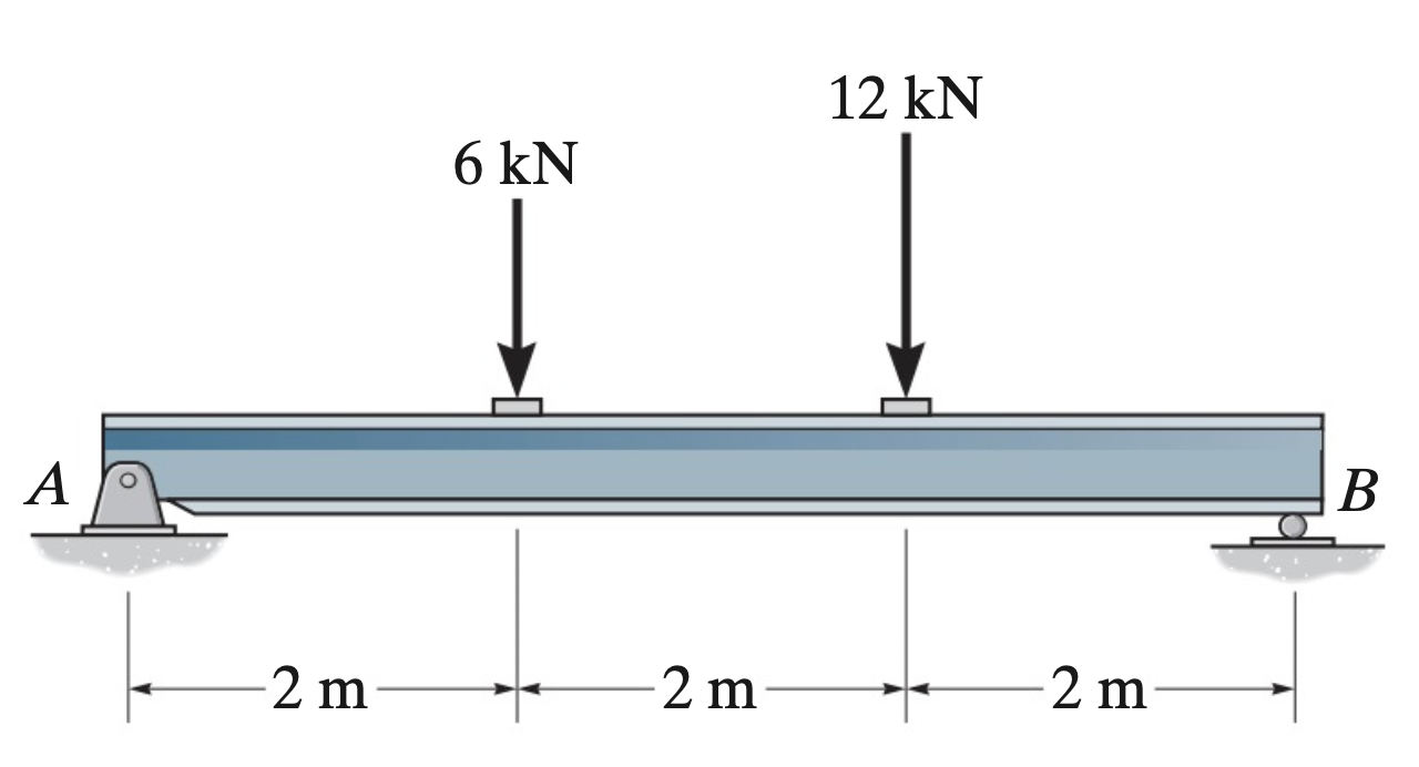
1) Solve for reaction at A:

With CW as positive, $\ \Sigma M_{B} = 0 = (A_{y})(6\ m) - (6\ kN)(4\ m) - (12\ kN)(2\ m)$

$A_{y} = 8\ kN$

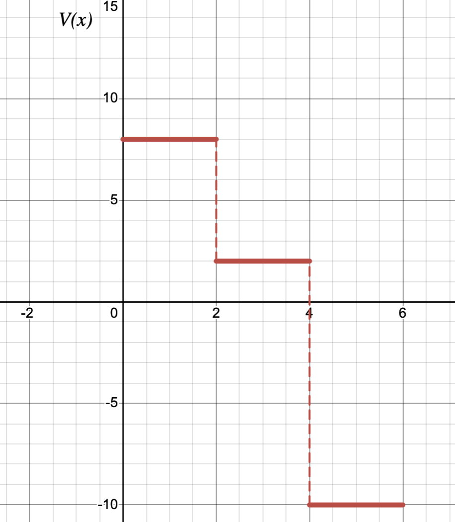
2) First cut between $0 \leq x < 2$:

$\Sigma F_{y} = 0 = A_{y} - V(x)$ → $V(x) = 8\ kN$

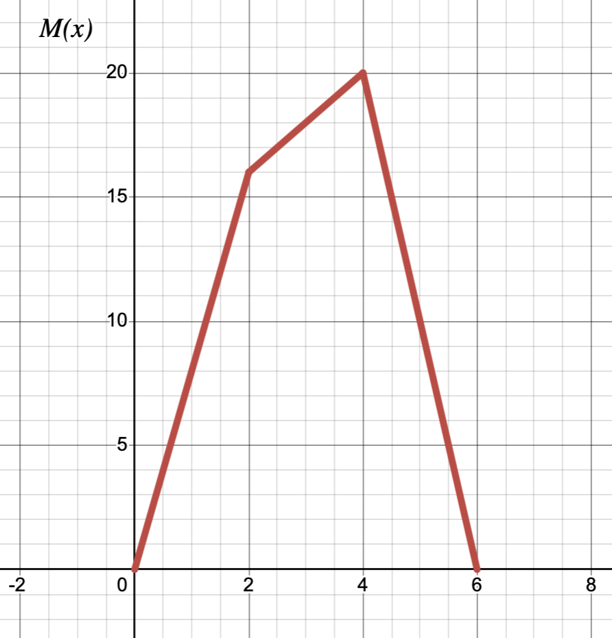
$\Sigma M = (A_{y})(x) = (8x)\ kN \cdot m$

3) Second cut between $2 \leq x < 4$:

$\Sigma F_{y} = 0 = A_{y} - 6\ kN\ - V(x)$ → $V(x) = 2\ kN$

$\Sigma M = (A_{y})(x) - (6\ kN)(x - 2) = (2x + 12)\ kN \cdot m$

4) Third cut between $4 \leq x < 6$:

$\Sigma F_{y} = 0 = A_{y} - 6\ kN - 12\ kN\ - V(x)$ → $V(x) = - 10\ kN$

$\Sigma M = (A_{y})(x) - (6\ kN)(x - 2) - (12kN)(x - 4) = ( - 10x + 60)\ kN \cdot m$

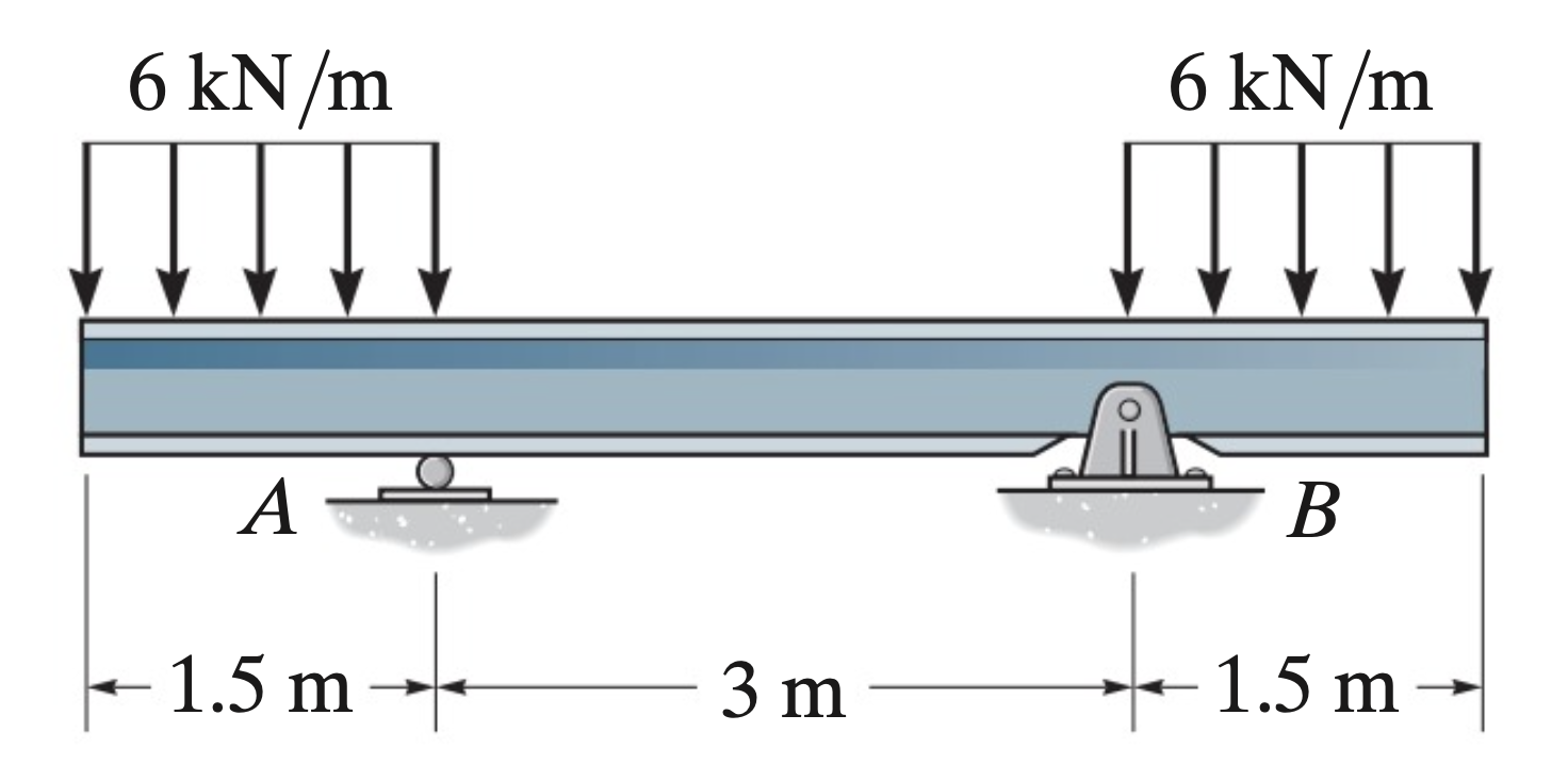
Example 2:

1) Simplifying distributed loads & solving for reaction A gives:

$F_{1} = F_{2} = A_{y} = B_{y} = 9\ kN$

$F_{1}$ and $F_{2}$ act at $x = 0.75\ m$ and $x = 5.25\ m$

3) First cut between $0 \leq x < 1.5$:

$\Sigma F_{y} = 0 = ( - 6\ kN/m)(x) - V(x)$

$V(x) = ( - 6x)\ kN$

$\Sigma M = ( - 6\ kN/m)(x)(\frac{x}{2}) = ( - 3x^{2})\ kN \cdot m$

4) Second cut between $1.5 \leq x < 4.5$:

$\Sigma F_{y} = 0 = ( - 9\ kN) + A_{y} - V(x)$

$V(x) = 0$

$\Sigma M = ( - 9\ kN)(x - 0.75) + (9\ kN)(x - 1.5)$

$\ \ \ \ \ \ = - 6.75\ kN \cdot m$

5) Third cut between $4.5 \leq x < 6$:

$V(x) = - 9\ kN\ + \ 9\ kN - 9\ kN - (6\ kN/m)(x - 4.5) = ( - 6x + 36)\ kN$

Using calculus for $M(x)$ → $\int_{}^{}V(x) = ( - 3x^{2} + 36x + C)\ kN \cdot m$

Solving for constant at integration since moment diagram is continuous at $x = 4.5\ m$:

$- 3{(4.5)}^{2} + 36(4.5) + C = 6.75$ → $C = \ 108$

$M(x) = \ ( - 3x^{2} + 36x + 108\ )\ kN \cdot m$

With all these equations for shear and moment, we can graph $V(x)$ and $M(x)$.