
Equivalent Force Systems and Distributed Loads
Introduction
Complex loading systems can often be simplified into a single equivalent force and couple moment acting at a point. An equivalent system produces the same external effect on a body as the original system with multiple forces and moments. In addition, distributed loads can be replaced by an equivalent concentrated force acting on the centroid of the distribution, making analysis easier.
Resultant Force
For any force system, . The location of the resultant force is . Using this method, the resultant force creates the same moment as the original system.
For 2D systems, , , and
Uniform Distributed Loading
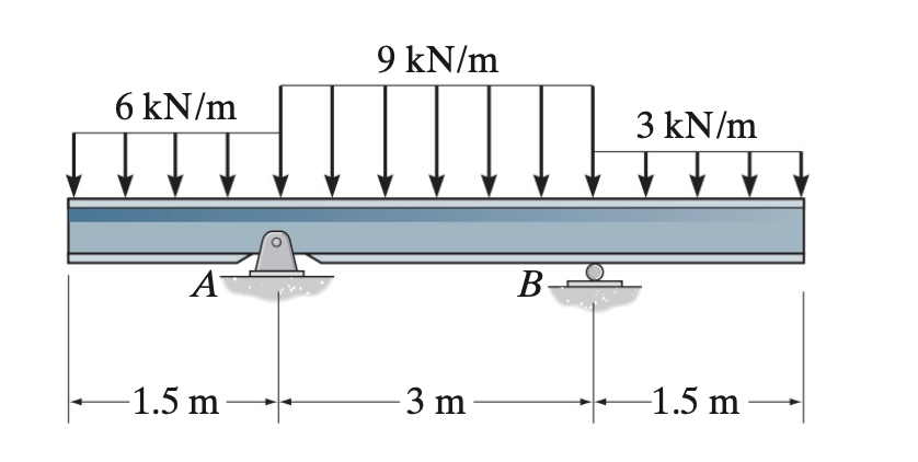
For a uniform distributed load, the resultant force is , where w is the intensity of the load in units of force per length. The resultant force acts at the midpoint of the distribution (.
Triangular Distributed Loading
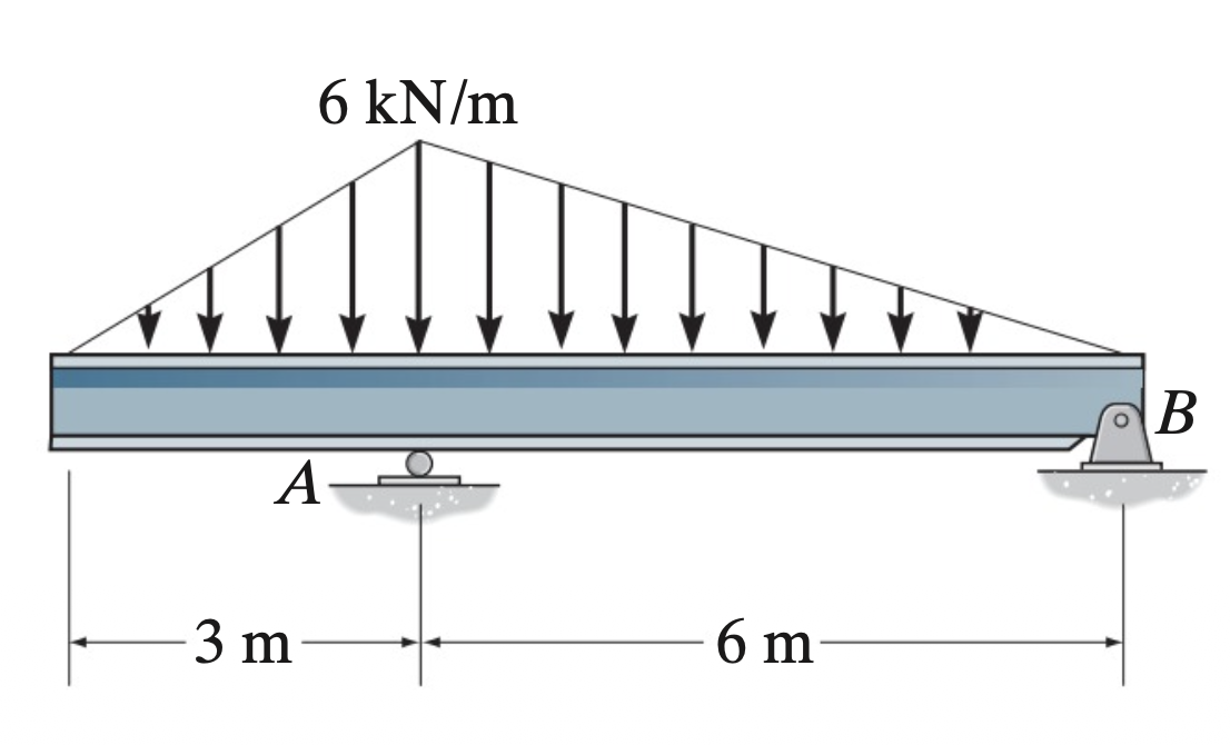
For a triangular distributed load, the resultant force is . The resultant force acts at length from the larger side.
Trapezoidal Distributed Loading
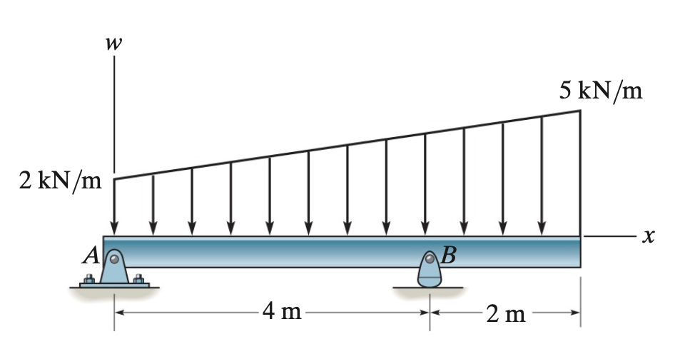
A trapezoidal distributed load is a combination of a uniform load and a triangular load. Split the trapezoid into a rectangle and triangle, find the resultant of each section, and sum forces. The rectangle has , the triangle has , and .
Function-Based Distributed Loading
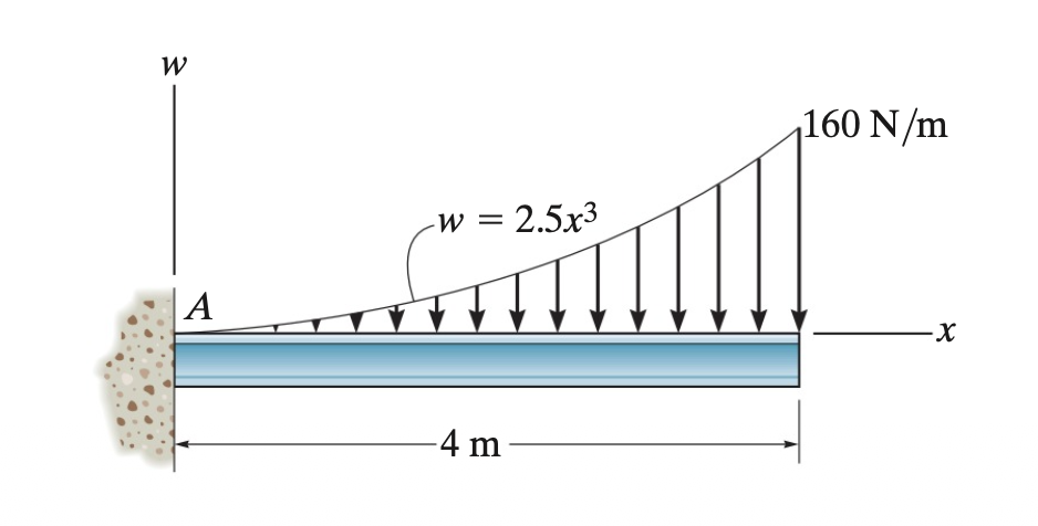
Loads can be described by a function . The resultant force is . This resultant force acts at a location (centroid) of .
Example 1:
Replace the forces with a single resultant force, and specify where it acts on AB, measured from point A
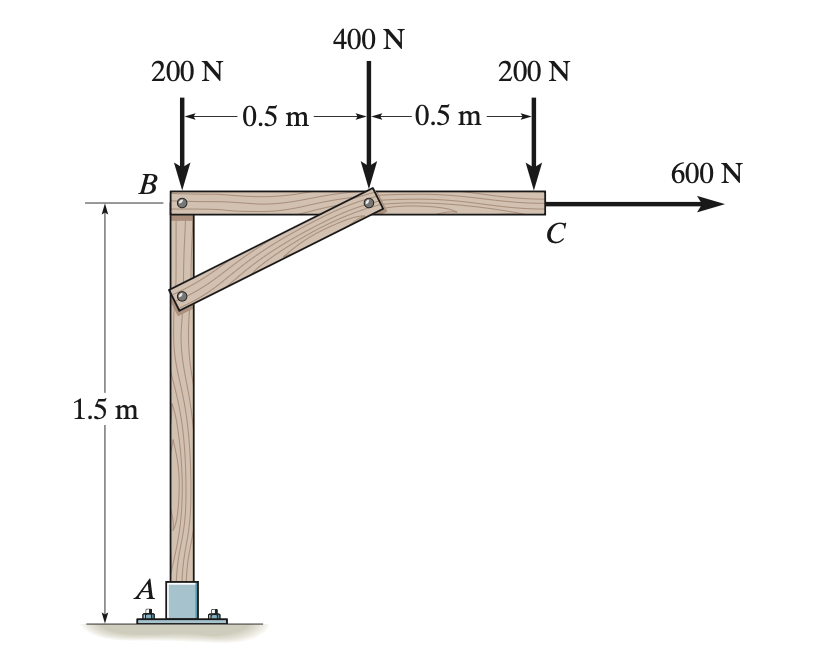
1) Sum Forces in x and y Directions:
2) Solve for Resultant Force:
down and to the right
3) Find where acts a distance from point A:
With clockwise as positive,
Since y distance from A is zero,
Example 2:
Find the resultant Force and Distance of Resultant Force from Point O
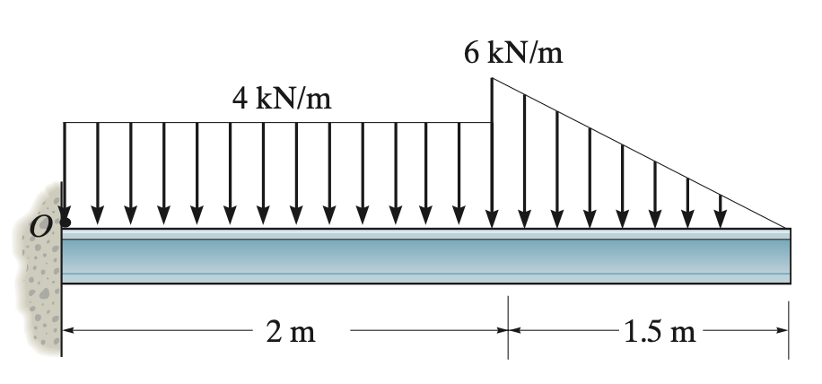
1) Break Up the Load into Rectangular and Triangular Distributed Loads to Solve for :
Rectangular:
Triangular:
2) Find where acts a distance from point O: