Contact Info

Location Engineering Building | room 332
Phone 435-797-1494
Contact Christian Bolander
Email christian.bolander@usu.edu

Hours

Mon–Thu	10am – 5pm
Fri	10am – 4pm

Drop-Ins Welcome!

Closed weekends and university holidays.

EMRC Algebra Review

The Equation of a Line

The equation of a line is generally given in slope-intercept form as

(1)

y = m x + b

where m is the slope and b is the y-intercept. We require two points of a line, given as (x1, y1) and (x2, y2), to find the slope and y-intercept when a line is given in slope-intercept form. Using these two points, the slope is calculated as

(2)

m = \frac{y_{2} - y_{1}}{x_{2} - x_{1}}

The y-intercept can then be found using either point as

(3)

b = y_{1} - m x_{1}

(4)

b = y_{2} - m x_{2}

A line can also be given in point-slope form as

(5)

y - y_{1} = m (x - x_{1})

In this case, we need only one point, (x1, y1), and the slope m to find any other point along the line. This form of the equation of a line is especially useful in certain circumstances in calculus when we talk about tangent lines.

Question 1. Before stall, the lift coefficient on an aircraft satisfies the relation

(6)

C_{L} (α) = C_{L 0} + C_{L, α} α

where $C_{L 0}$ is the lift coefficient at zero-degrees angle of attack and $C_{L, α}$ is the change lift with angle of attack. Determine $C_{L 0}$ (dimensionless) and $C_{L, α}$ (in per-degrees) if the lift coefficient is known at the following two points.

$α$ , degrees	$C_{L} (α)$
-5	-0.2
3	0.25

Find the angle of attack at which the aircraft generates no lift (the zero-lift angle of attack) and plot the lift curve.

Quadratic Equations and Their Solutions

A quadratic equation is a second-degree polynomial and takes the form

(7)

a x^{2} + b x + c = 0

Many times they will also appear in factored form as

(8)

(x + c) (x + d) = 0

This form is useful for solving quadratic equations. Quadratic equations have solutions that come in pairs that sometimes contain imaginary numbers.

Quadratic equations can be solved in many different ways. Many of the methods that are used to solve quadratic equations take advantage of the zero-product property. The zero-product property says that any value multiplied by zero has a product of zero. With a quadratic equation factored as in Eq. (8), we can then see that with x = −c and x = −d, one of the factors is zero and therefore the product of the factors must also be zero. When c = d, we call the factored form of the quadratic a perfect square.

One of the most common methods used to solve quadratic equations is by using the quadratic formula. The formula is given as

(9)

x = \frac{- b \pm \sqrt{b^{2} - 4 a c}}{2 a}

which gives two solutions by virtue of the $\pm$ in the numerator. This method works for all quadratic equations, but the methods that follow introduce principles that allow for solving higher-order polynomials.

Another method is to solve the quadratic equation using grouping. The idea of grouping is to split the linear term, b, into two factors that multiply to become the product ac. By doing so we can create a situation in which we can solve the equation by using the zero-product property. In short, this method is approached using the following steps:

Find the factors of the product ac that add together to become b
Separate b into those factors to yield an equation of the form $a x^{2} + b_{1} x + b_{2} x + c = 0$
Find a common factor between two pairs of the four terms
Factor the equation and use the zero-product property to solve

Finally, we can solve quadratic equations by completing the square. Completing the square can only be used when a = 1. When completing the square, we again manipulate the linear term to create a perfect square. This method has the follow steps:

Move the constant term c to the right-hand side
Add ${(\frac{b}{2})}^{2}$ to both sides and simplify the right-hand side
The left-hand side can be made a perfect square
Take the square root of both sides and solve for x (remember to add a ± on the right-hand side!)

Question 2. A projectile is fired in the vertical plane with its height given by the equation

(10)

h (t) = 96 t - 16 t^{2}

Find the time t when h = 80 ft [1].

Complex Numbers

We regularly deal with real numbers, which include the positive and negative integers of the number line, the rational numbers (non-infinite decimals), and every number in between. A complement to the real numbers are complex numbers, which are used often in engineering. A complex number has both real and imaginary parts. The imaginary number i is defined as

(11)

i = \sqrt{-1}

Therefore, we note that

(12)

i^{2} = {(\sqrt{-1})}^{2} = -1

Using the imaginary number i, we can define a complex number as

(13)

z = a + b i

A complex number can be plotted in the complex plane with a = 3 and b = 1 as

$A point in the complex plane.$

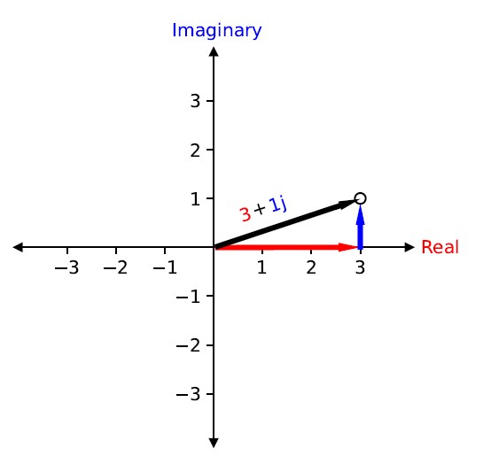
Figure 1. A point in the complex plane.

These numbers can be manipulated using similar principles as the real numbers. For example, when adding or subtracting complex numbers, simply add or subtract the real parts and imaginary parts separately. That is,

(a + b i) + (c + d i) = (a + c) + (b + d) i

(a + b i) - (c + d i) = (a - c) + (b - d) i

Multiplying a complex number by a real number utilizes the distributive property, becoming

c (a + b i) = (c a) + (c b) i

We can use the definition in Eq. (12) and distribution to find that multiplying a complex number by another complex number yields

(a + b i) (c + d i) = (a c) + (a d) i + (b c) i + (b d) i^{2} = (a c - b d) + (a c + b c) i

At times division of complex numbers may also be required. To do so, we must introduce the concept of a complex conjugate. The complex conjugate of a complex number represents a reflection of the complex vector, as shown in Fig. 1, across the real axis. Thus, given the complex number $z = a + b i$ , its complex conjugate is $z̅ = a - b i$ and vice versa. Multiplying a complex number by its complex conjugate results in a purely real number. Therefore, when dividing a complex number into another complex number, we multiply the numerator and denominator by the complex conjugate of the denominator.

\frac{a + b i}{c + d i} = \frac{a + b i}{c + d i} (\frac{c - d i}{c - d i})

= \frac{(a c + b d) + (b c - a d) i}{(c^{2} + d^{2}) + (c d - c d) i}

= \frac{(a c + b d) + (b c - a d) i}{c^{2} + d^{2}}

Since complex numbers can be treated as a vector in the complex plane (see Fig. 1), we can express complex numbers as a magnitude and direction in that plane. The magnitude of the complex number

(14)

|z| = \sqrt{a^{2} + b^{2}}

and the angle that it makes with respect to the real axis is

(15)

θ = atan2 (\frac{a}{b})

This can sometimes be written in polar form as

(16)

a + b i = |z| < θ

Finally, complex numbers can be written in terms of an exponential using Euler’s formula. Euler’s formula states that

(17)

cos θ + (sin θ) i = e^{θi}

and therefore by writing our complex number as

z = |z| cos θ + (|z| sin θ) i

we can see that, in exponential form,

(18)

z = |z| e^{θ i}

Question 3. An electric motor has a resistance R = 10 Ω and an inductance of L = 0.025 H. If the motor is connected to a 110 V, 60 Hz source, find the current I = V/z. Note that z = zR + zL, zL = (ωL)i, zR = R, and ω = 2πf where f is the frequency of the source. Give your answer as a complex number, in polar form, and in exponential form [1].

Systems of Equations

Engineers are often required to deal with systems that have inter-related components that are dependent on certain physical properties. In these situations, these system components can be described using a system of equations.

An important principle of dealing with systems of equations is understanding the number of solutions that a particular system has. For example, for a system given by

2 x + y = 15

3 x - y = 5

we may expect to find a unique (x, y) coordinate pair that satisfies both equations. Any ordered pair that satisfies the system of equations is considered a solution to that system. In fact, there may be one solution, many solutions, infinitely many solutions, or no solutions at all to a system of equations! Here we will focus on systems of linear equations, where we may make some notes on the general behavior of the systems.

When determining the number of solutions a system of linear equations has, we may examine the number of equations and the number of unknowns. In general, a system with fewer equations than unknowns has either infinitely many solutions or no solution. We refer to this kind of system as an underdetermined system. A system with more equations than unknowns has no solution and is called an overdetermined system. Finally, a system with the same number of equations as unknowns generally has a single unique solution. Specific values for the coefficients in a system of linear equations can disrupt these general behaviors.

We can solve systems of equations using many techniques. Some of these solutions methods will be explored in this section and some will be given once we have introduced the concept of matrices. One helpful way to solve systems that is particularly helpful with 2 unknowns is using a graphical approach. Any intersections of the equations is a solution to the system.

Systems of linear equations can also be solved using the substitution method. This method solves one equation for one of the variables and then substitutes that variable into the next equation. This process is repeated until a solution for one variable is obtained, at which point that solution can be used in previous equations to yield the solution for the system.

The final way to solve systems of equations that will be discussed here is using the method of elimination. By adding equations together that have opposite coefficients in front of the same variable, that variable will be eliminated from the resulting equation. This process can be repeated as many times as necessary using other pairs of equations to yield systems with a reduced number of equations and unknowns.

Question 4. For the block shown in Fig. 2 to remain motionless, the following equations must be satisfied

{-T}_{1} cos(20°) + T_{2} cos(50°) = 0

T_{1} sin(20°) + T_{2} sin(50°) = 30

Solve for the tension in the ropes (given by T1 and T2) using the graphical approach, substitution, and elimination.

$System of ropes holding a block$

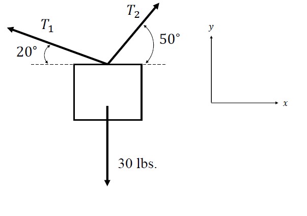
Figure 2. System of ropes holding a block.

Matrices and Matrix Operations

A matrix is a rectangular array of numbers where the rows of the matrix are aligned horizontally and the columns of the matrix aligned vertically. Each of the entries in the matrix are called elements of the matrix. As an example, a matrix A can be written as

(19)

A = [\begin{matrix} a_{11} & a_{12} & \dots & a_{1 n} \\ a_{21} & a_{22} & \dots & a_{2 n} \\ ⋮ & ⋮ & ⋱ & ⋮ \\ a_{m 1} & a_{m 2} & \dots & a_{m n} \end{matrix}]

The dimensions of a matrix, written as m×n or m rows and n columns, are very important when dealing with matrix operations.

The first of these matrix operations are addition and subtraction. Adding or subtracting two matrices A and B is defined as the addition and subtraction of corresponding elements

(20)

A + B = a_{i j} + b_{i j}

where ij indicate the i^th row and j^th column of the corresponding matrix. Therefore, addition and subtraction of matrices requires that each matrix and the resulting matrix have the same dimension. Matrix addition and subtraction is commutative (order doesn’t matter) and associative (grouping doesn’t matter).

Scalar multiplication of matrices is also a defined matrix operation. When a matrix is multiplied by a scalar, the elements of the matrix are each multiplied by the scalar. Thus,

(21)

c A = [\begin{matrix} c a_{11} & c a_{12} & \dots & c a_{1 n} \\ c a_{21} & c a_{22} & \dots & c a_{2 n} \\ ⋮ & ⋮ & ⋱ & ⋮ \\ c a_{m 1} & c a_{m 2} & \dots & c a_{m n} \end{matrix}]

Scalar multiplication of a matrix is distributive, meaning, for example, that $a (A + B) = a A + a B$ .

Although the matrix operations we have explored until now have been analogous to traditional arithmetic techniques, matrix multiplication requires additional tools and techniques. The result of the product of two matrices is only defined if the inner dimensions of those matrices is the same. In the case of the product of a matrix A with dimension 3 × 4 and a matrix B with dimension 4 × 2, the inner dimension is the columns of the matrix A and the rows of the matrix B. The matrix resulting from the product of A and B will have dimensions equal to the outer dimensions of the component matrices. In our example, C = AB will have dimension 3 × 2.

To calculate the value of an element cij in the product of matrix A and matrix B, we take the ith row of matrix A and multiply it by the jth row of matrix B. This multiplication is carried out by multiplying the first element in the ith row of A by the first element in the jth column of B and adding the result to the product of the next elements in each. This pattern is repeated until all of the elements in the ith row of A and jth row of B are accounted for. Symbolically, this process is given by

(22)

[\begin{matrix} a_{i 1} & a_{i 2} & \dots & a_{i n} \end{matrix}] [\begin{matrix} b_{1 j} \\ b_{2 j} \\ ⋮ \\ b_{m j} \end{matrix}] = a_{i 1} b_{1 j} + a_{i 2} b_{2 j} + \dots + a_{i n} b_{m j}

By repeating this process for each element cij in the product matrix, C can be constructed.

Note that matrix multiplication is associative (grouping doesn’t matter) and distributive (groups distribute), but not commutative (order does matter!). Systems of equations, as described in the previous section, are readily described using matrix notation. For example, a two-loop circuit can be described as a system of equations using Kirchoff’s Voltage Law as

a I_{1} + b I_{2} = e

c I_{1} + d I_{2} = f

where a, b, c, and d are taken from the resistance of conductors, I1 and I2 are currents in the circuit, and e and f are voltage from two supplies. The coefficients on the left-hand side of this system can be rearranged into a matrix

A = [\begin{matrix} a & b \\ c & d \end{matrix}]

while the coefficients on the right-hand side can be expressed as the vector

B = [\begin{matrix} e \\ f \end{matrix}]

Finally, matrix multiplication can show us that

A [\begin{matrix} I_{1} \\ I_{2} \end{matrix}] = B

is equivalent to the two-loop circuit system described above.

Question 5. Describe the system in Question 4 as a matrix multiplication problem $A x = B$ . Then, solve for the tension in the ropes using the following formula

(23)

[\begin{matrix} T_{1} \\ T_{2} \end{matrix}] = \frac{1}{-cos(20°) sin(50°) - cos(50°) sin(20°)} [\begin{matrix} sin(50°) & -cos(50°) \\ sin(20°) & -cos(20°) \end{matrix}] [\begin{matrix} 0 \\ 30 \end{matrix}]

Sequences and Series

A sequence is a function whose domain is given by the positive integers and whose range is an ordered list of numbers. Rather than listing the terms in this list explicitly, we can describe a sequence using an explicit formula, such as

a_{n} = 2^{n}

meaning that the nth term in the sequence is given by 2n. Sequences can be either finite or infinite, which is indicated using ellipses at the end of the sequence, as in

\{1, 2, 3, …, 10, …\}

Infinite

\{1, 2, 3, …, 10\}

Finite

Sequences can also be recursive, which means that each term is defined using the preceding terms. The initial term(s) in a recursive formula must always be stated explicitly. An example of a recursive formula is

a_{1} = 1

a_{n} = 2 a_{n - 1}

An important example of a recursive formula is n factorial, n!, which is defined recursively as

0! = 1

1! = 1

n! = n (n - 1) (n - 2) \dots (2) (1)

, for n ≥ 2

We must take the time to define what it means for a sequence to converge. For a sequence to converge, we say that there exists a limit L such that for some index N the following holds:

(24)

|a_{n} - L| < ε

, for all n < N

for all values of ε > 0. A sequence is called a divergent sequence if it does not converge.

There are several important types of sequences. The first of these is an arithmetic sequence, which changes by a constant amount with each subsequent term. That is,

\{a_{n}\} = \{a_{1}, a_{1} + d, a_{1} + 2 d, a_{1} + 3 d, \dots\}

where d is the constant difference between terms. Arithmetic sequences will therefore always be linear and their explicit formula is

(25)

a_{n} = a_{1} + (n - 1) d = a_{n - 1} + d

, n ≥ 2

Geometric sequences are sequences where each subsequent term is multiplied by a common ratio. We can write these sequences as

a_{n} = \{a_{1}, a_{1} r, a_{1} r^{2}, a_{1} r^{3}, \dots\}

The common ratio can be found by dividing any term by the previous term. The recursive formula for a geometric sequence is given by

(26)

a_{n} = r a_{n - 1}

, n ≥ 2

and the explicit formula is

(27)

a_{n} = a_{1} r^{n - 1}

By summing the terms in a sequence, we define a series. Mathematically we denote a series using summation notation, such that

(27)

s = \sum_{k = 1}^{n} a_{k}

Thus, an arithmetic series is given by

(28)

s = \sum_{k = 1}^{n} a_{1} + (k + 1) d

and a geometric series is given by

(29)

s = \sum_{k = 1}^{n} a_{1} r^{k - 1}

The arithmetic series never converges, since each term increases by a constant factor. A geometric series, however, does converge, so long as |r| < 1.

Question 6. Write an explicit formula for the following sequence and determine if it is convergent.

(30)

\{2, 1.8, 1.62, 1.458, …\}

Question 7. Under what conditions is the following series convergent? Assume An are constants.

(31)

a_{n} = \sum_{n = 1}^{N} A_{n} sin(nθ)

References

[1] Engineering mathematics (egr 1010) topics and materials. https://engineering-computer-science.wright.edu/research/engineering-mathematics-topics-and-materials. Accessed: 2022-08-04.